
The Curve Stableswap (V1) is the basis for the whole curve ecosystem. It provides the building blocks on which Curve V2 and crvUSD are built. It also provides fees which give CRV fundamental value. So it’s important to understand how the system works to understand the further developments that have come since then.
The idea behind StableSwap’s development was to create a place where assets which are softpegged to each other (eg. USDC:USDT) can be traded without incurring large amounts of slippage. This wasn’t possible at the time of it’s development. Stablecoins and likekind assets had to be traded on centralised exchanges.
Overview of Pools
The design of the system revolves around smart contracts called pools which hold either 2 or more likekind assets (eg. USDC, USDT) see fig. 1. Apart from holding assets, pools also implement very important functionality:
- Adding and removing liquidity from a pool. Allowing the user to receive a share of the fees generated from exchanges (swaps) in the pool. See fig. 2
- Exchanging between assets in the pool. See fig. 3
- Withdrawal of fees for veCRV holders
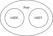
Fig.1: Diagram of tokens held by a pool
Fig. 2 shows the how the pools change when a user deposits their coins to these pools. They deposit both coins and receive tokens representing their share of deposited liqudity in the pool (LP Tokens). When no swaps have occured in the pool, 2 LP tokens will be worth 1 USDT and 1 USDC (2 LP tokens = $2).
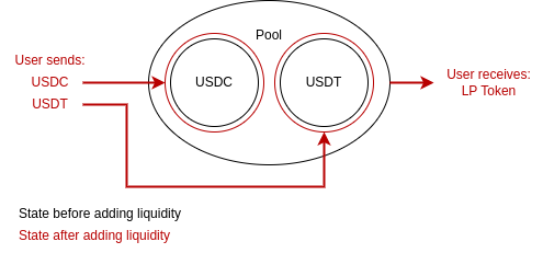
Fig.2: State change of user adding liquidity to a pool
As swapping occurs (Fig. 3), the pool generates fees. The normal swap fee is 0.04% which is split evenly between the LPs (0.02%) and the veCRV holders (0.02%), although some pools have different fees. The veCRV fees are transferred out of the pool frequently but the LP fees are left in the pool forever. As each LP token represents an even share of assets in the pool this has interesting consequences:
- As swaps happen, assets in the pool increase from the generated fees which causes the LP token to be worth more and more over time (up only!, see the charts on https://curve.fi/#/ethereum/pools/3pool/deposit for an example of LP token price increasing)
- If you deposit the same amount of coins to a pool when it is created and then after 100 swaps have occured, you will get less LP tokens in the 2nd deposit as fees have increased the value of the LP tokens.
This is all assuming the assets in the pool do not depeg from each other permanently. Although any temporary depegs can prove to be significantly profitable for LPs.
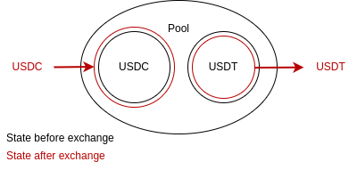
Fig.3: State change of user exchanging USDC for USDT
You can deposit any variation of token amounts you wish (eg. 0.1 USDC, 1000 USDC). You will get bonuses for depositing more of the asset with a lower amount in the pool. Withdrawals happen by the user receiving an even split of assets in the pool, but they can opt to withdraw to a single coin with the protocol first withdrawing and then swapping after in a single transaction. The smart contracts natively build this functionality into pools.
Deriving the Stableswap Invariant
When one asset is swapped for another the price of both assets needs to be known. This may seem like a simple problem or fact to know, but within smart contracts this is actually harder than many realise. We need a formula to always allow these assets to swap between each other so the market can find it’s own price. The strongest way to find the correct price is to let the market forces do it for us themselves. Arbitrage and money is a very powerful motivator. So we start with a simple formula. We assume that the prices of the assets in the StableSwap pools should be stable, ie. not changing. We get the formula below, let’s call it the constant sum invariant (invariant is a fancy name for a formula that is constant):
$$\sum x_i = \textrm{const}$$
Where \(x_i\) is the balance of each coin in the pool, ie from fig 1. \(x_0\) would be balance of USDC and \(x_1\) would be the balance of USDT. The formula above means that if we have 10 USDT and 10 USDC then the sum is always 20. We could allow these to be locked at a constant 1:1 price as shown in the constant sum above, but if they aren’t worth exactly 1:1, even if 1 USDC is worth 0.999 USDT, the pool will be drained. People will swap their USDC for USDT through the pool because they can swap a lower worth asset for free for a higher worth asset. The pool will be left with 20 USDC and 0 USDT. This is a valid state (\(s_i\)) for the constant sum formula. For a constant sum pool all the following states would be valid:
| \(s_1\) | \(s_2\) | \(s_3\) | \(s_4\) | \(s_5\) | |
| USDC | 10 | 15 | 5 | 0 | 19.2 |
| USDT | 10 | 5 | 15 | 20 | 0.8 |
| Sum (USDC + USDT) | 20 | 20 | 20 | 20 | 20 |
Table 1: Possible states of the constant sum formula
When we graph this it looks like the following shown in fig. 4.
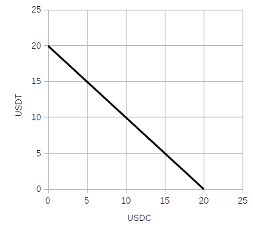
Fig.4: Constant sum formula
So we need something better. Instead of adding, let’s try multiplying. We will call it a constant product invariant. This was the formula made famous by this post by Vitalik. This was also formula which was the backbone of Uniswap’s V1 and V2. In mathematics terms it looks like the following:
$$\prod x_i = \textrm{const}$$
If we continue with the USDC, USDT example it means that the amount of USDC multiplied by the amount of USDT stays constant. So if we have 10 USDT and 10 USDC the constant is 100. It’s important to define the midpoint of this formula (where the two balances are equal in $ value). If we have the midpoint as a constant of 100, then the following states are possible:
| \(s_1\) | \(s_2\) | \(s_3\) | \(s_4\) | \(s_5\) | |
| USDC | 1 | 2 | 10 | 19 | 10000 |
| USDT | 100 | 50 | 10 | 5.26 | 0.01 |
| Prod (USDC * USDT) | 100 | 100 | 100 | 100 | 100 |
Table 2: Possible states of the constant product formula
Interestingly with this formula we can get very large amounts of USDC and very small amounts of USDT without the values ever going to 0 as seen in Fig. 5.
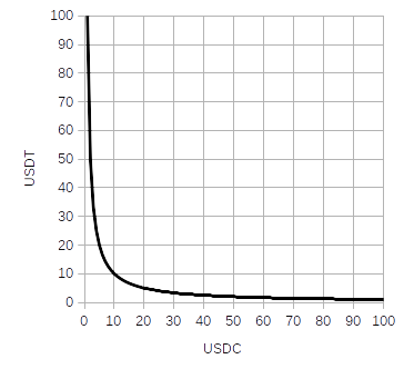
Fig.5: Constant product formula
This formula will never be able to get a 0 balance for USDC or USDT like the constant sum formula could. This is a big positive. We always want to be able to swap for a price, no matter what that price is. But it’s also bad for stablecoins and pegged assets. If a pool has 10 USDT and 10 USDC and we want to swap 1 USDT for USDC we get a very bad price, we only get $0.91 cents of USDC. Here’s how it works:
- The pool starts with 10 USDT, 10 USDC, with a constant product of 100
- We give 1 USDT to the pool, the pool now has 11 USDT
- The pool uses the formula: $$\textrm{USDC}*\textrm{USDT} = 100$$
Therefore: $$\textrm{USDC} = \frac{100}{\textrm{USDT}}$$
Subtituting for USDT =11:
$$\textrm{USDC} = \frac{100}{11}=9.09$$ - The pool currently has 10 USDC, and it knows it needs 9.09 to satisfy the constant product formula, so it knows to send us:
$$10-9.09 = 0.91 \textrm{USDC}$$
This formula works well for assets with very little pricing information available, eg. memecoins when they first launch. But it does not work well for assets which should be tightly pegged to each other most of the time. We want something that will give us liquidity at any price (never have 0 balance) and also give us good prices when close to the midpoint. We need to be able to sway 10-30% from the midpoint and still get close to 1:1 swaps. From the whitepaper:
We are looking for some invariant which is relatively flat near balance (price changes slowly, the graph is very close to the straight line, likely a “zoomed in” hyperbola), however shifting towards the constant-product invariant as the portfolio becomes more imbalanced (e.g. closer to the axes).
Michael Egorov: StableSwap Whitepaper, 2019
Perhaps we could use the constant product and constant sum together in some way? If we have a pool and the price of all assets in the pool are exactly the same (eg, 1 USDC = 1 USDT) then the following invariants hold:
$$ \sum x_i = D$$ $$\prod x_i = \left( \frac{D}{n} \right)^n$$
Where \(n\) are the number of coins in the pool eg. for the USDC, USDT example this is 2. \(i\) is the coin index eg. 0 refers to USDC, 1 refers to USDT. Now we can think of the constant sum invariant as giving infinite leverage as it will give us the same price no matter how much of either coin is left. We can also think of the constant product invariant as giving 0 leverage because it doesn’t allow a close to 1:1 price when the pool is perfectly balanced. We want something between these extremes, so curve ingeniously introduces a term for leverage, let’s call it \( \alpha\) (it’s defined as \(\mathcal{X}\) in the whitepaper, but that’s too close to \(x\) for me, and it’s easy to get confused by it). Let’s also multiply the constant sum invariant by \( \alpha\), this will mean when \( \alpha\) = 0 the constant sum will be turned off, this will work well when we add this to the constant product invariant: $$ \alpha \sum x_i = \alpha D$$ Let’s add this to the constant product invariant: $$\alpha \sum x_i + \prod x_i = \alpha D + \left( \frac{D}{n} \right)^n$$
This new invariant gives us the constant sum invariant when \( \alpha = \infty\) as the value of the constant product will be very small compared to constant sum. This is what we want. Now at this point in the whitepaper they redefine \( \alpha \) to be \(\alpha = \alpha D^{n-1}\). This is to stop a problem. Currently without this change, as our balances increase, the leverage needs to as well. If you have 10 USDC, 10 USDT, \( \alpha \) = 10 the contribution from the constant sum and constant product is actually equal to 1000 USDC, 1000 USDT, \( \alpha \) = 1000. It makes more sense if the magnitude of \(\alpha \) does not need to increase as the balances increase, therefore we change the full invariant (we will call it ComboSwap) to:
$$\alpha D^{n-1} \sum x_i + \prod x_i = \alpha D^n + \left( \frac{D}{n} \right)^n$$
Below we can see how this ComboSwap compares to the constant sum and constant product invariants with different levels of leverage. See that when \( \alpha\) gets close to 0 it starts to resemble the constant product and resembles the constant sum when \( \alpha\) increases.
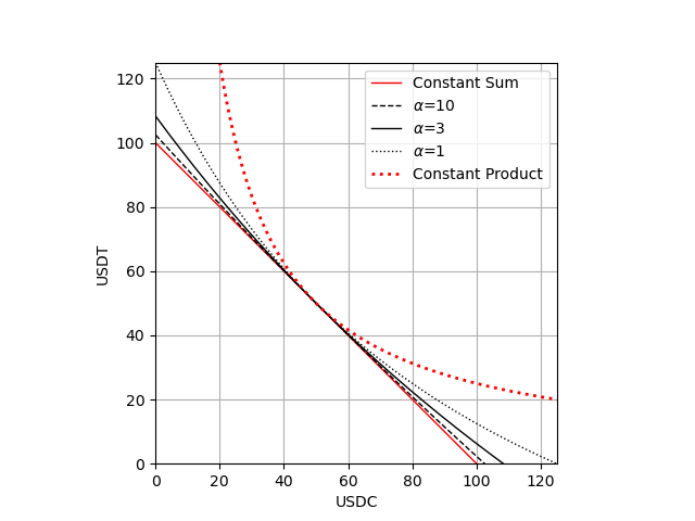
Fig.6: ComboSwap vs. Constant Sum and Constant Product
The above function still has some downsides.
- It does not give liquidity at every price, eg. if \(\alpha = 10\) and there is 125 USDC there is 0 USDT in the pool
- It gives bad prices for stablecoins if it’s not in perfect balance, eg. if \(\alpha = 10\) and there is ~40 USDC and ~60 USDT then you get 1.15 USDT for every 1 USDC you trade through the pool. This is not ideal, if pools are 60%/40% they should still be in nearly perfect equilibrium.
This is why the whitepaper makes \(\alpha\) dynamic. Currently we have something half between constant product and constant sum at all points. What we really want is something that is equal to constant sum when pools are close to balanced, and equal to constant product when pools are out of balance at the limits. This is why the following substitution for \(\alpha\) is made:
$$\alpha = \frac{A \prod x_i}{{(D/n)}^{n}}$$
Subtitute for \(\alpha\) in ComboSwap and simplify to get the complete StableSwap invariant that is used within Curve:
$$An^{n} \sum x_i + D = ADn^{n} + \frac{D^{n+1}}{n^{n} \prod{x_i}}$$
This meets all the desired criteria by giving stable prices when liquidity is close to balanced while also giving prices at every point to infinity.
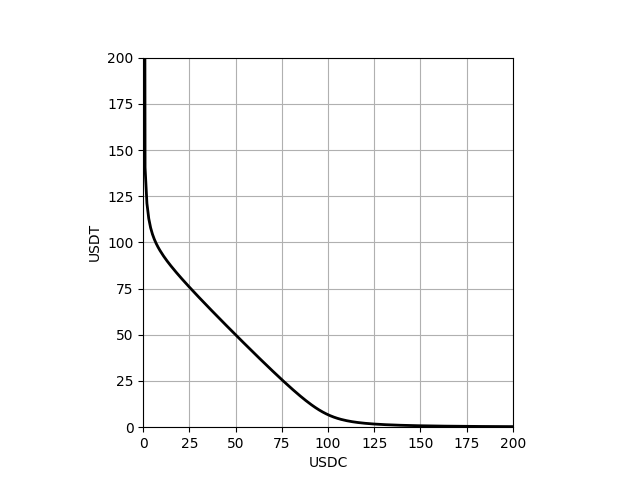
Fig.7: StableSwap
The amplification factor of the Stableswap Invariant (\(A\))
In all pools there will be an amplification factor (\(A\)), it is a constant value, eg. in 3pool \(A = 2000 \). The higher the \(A\) the tigher the prices for longer along the curve. Higher \(A\) values also mean the curve will be flatter in the middle and resemble the constant sum more closely. The lower \(A\) becomes the more it will resemble the constant product invariant.
Pools which can have a higher correlation with each other (eg. USDT/USDC) can have a higher A as it allows for closer to 1:1 pricing further along the curve as pools become inbalanced. For example if \(A=10\) prices are close to 1:1 up until 75%USDT/25%USDC, but if \(A=100\) prices are close to 1:1 up until 90%USDT/10%USDC. See below:
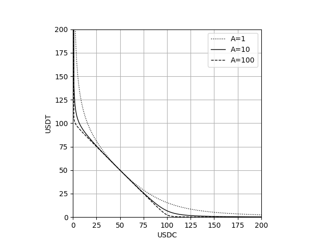
Fig.8: StableSwap amplification coefficient changes
The amplification factor of a pool can be changed by the Curve DAO at anytime by a majority vote.
The parameter \(D\) and it’s calculation
The \(D\) parameter in the invariant is defined in the whitepaper as the following:
The constant \(D\) has a meaning of the total amount of coins when they have an equal price.
Michael Egorov: StableSwap Whitepaper, 2019
So the \(D\) parameter essentially represents total value of all coins in the pool. To find it’s value we have to use Newton’s Method to update from the previous value (\(D_{prev}\)) to the current value (\(D\)) before each swap in the pool. Newton’s method is defined as: $$D = D_{prev}-\frac{f(D_{prev})}{f'(D_{prev})}$$
So let’s go through how this works. We take the StableSwap invariant put everything on one side and call it \(f(D)\): $$f(D) = ADn^{n} + \frac{D^{n+1}}{n^{n} \prod{x_i}} – D – An^{n} \sum x_i$$
Then we take the derivative of this to find \(f'(D)\): $$f'(D) = An^{n} + \frac{(n+1)D^{n}}{n^{n} \prod{x_i}} – 1$$
Then we substitute everything in and we can iterate with this equation to find the current \(D\) based on the previous value \(D_{prev}\):
$$D = D_{prev} – \frac{AD_{prev}n^{n} + \frac{D_{prev}^{n+1}}{n^{n} \prod{x_i}} – D_{prev} – An^{n} \sum x_i}{An^{n} + \frac{(n+1)D_{prev}^{n}}{n^{n} \prod{x_i}} – 1}$$
This is very messy. So they make a few simplifications to make it nicer to compute. Let’s define a few different things: $$S = \sum x_i \quad \quad \quad \quad P = \frac{D_{prev}^{n+1}}{n^n \prod x_i}$$
Expanding and simplifying Newton’s iterative equation for \(D\)
Using the substitutions above we get the following equation which is slightly easier to read: $$D = D_{prev} – \frac{An^{n}D_{prev} – D_{prev} – An^{n} S + P}{An^{n} + \frac{(n+1)P}{D_{prev}} – 1}$$ The only slightly confusing part of this substitution is that: $$ \frac{(n+1)D_{prev}^{n}}{n^{n} \prod{x_i}} = \frac{D_{prev}((n+1)D_{prev}^n)}{D_{prev}(n^n \prod x_i)} = \frac{(n+1)D_{prev}^{n+1}}{D_{prev}(n^n \prod x_i)} = \frac{(n+1)P}{D_{prev}}$$ We can simplify the Newton’s method further from here by getting rid of the \( D_{prev}\) out the front: $$D = \frac{D_{prev}(An^{n} + \frac{(n+1)P}{D_{prev}} – 1)}{An^{n} + \frac{(n+1)P}{D_{prev}} – 1} – \frac{An^{n}D_{prev} – D_{prev} – An^{n} S + P}{An^{n} + \frac{(n+1)P}{D_{prev}} – 1} $$ $$ D= \frac{D_{prev}(An^{n} + \frac{(n+1)P}{D_{prev}} – 1) -(An^{n}D_{prev} – D_{prev} – An^{n} S + P)}{An^{n} + \frac{(n+1)P}{D_{prev}} – 1}$$ If you expand from here you’ll get: $$D = \frac{nP + An^n S}{An^n – 1 + (n+1)\frac{P}{D_{prev}}}$$ Then by multiplying top and bottom by \( D_{prev} \) we get the final form of the equation, shown below.
Expanding and simplifying using the process above we get the following form of the equation which is used in the smart contracts: $$D = \frac{D_{prev}(nP + An^n S)}{(n+1)P + D_{prev}(An^n-1)}$$
This equation is for Newton’s method, so we start with the previous value of \( D \) from the last swap and then iteratively calculate the current value of \( D \). This should converge to a new value within 4 iterations. Below you can find an example if you wish to see how the calculation is made.
Example D iterative calculation
Let’s start with a pool with two coins with balances of 900.1 USDT, and 1100 USDC. In the pool \( A = 100 \). Someone just swapped 100 USDC for 99.9 USDT so let’s calculate the current \( D \). Let’s assume that \( D=2000 = 1000 \text{USDT} + 1000\text{USDC} \) before the swap because the pool was perfectly balanced. All the parameters for our Newton’s equation first iteration are therefore the following:
$$ D_{prev} = 2000, \: A=100, \: n = 2, \: S = 900.1 + 1100 = 2000.1 $$$$ P = \frac{2000^{2+1}}{2^2 (900.1*1100)} = 2020.0$$For our first iteration we substitute in all the values we know to the equation for the current value of \( D \) found above:
$$D = \frac{D_{prev}(nP + An^n S)}{(n+1)P + D_{prev}(An^n-1)}$$ $$D = \frac{2000((2)(2020) + (100)(2)^2 (2000.1))}{(2+1)(2020) + 2000((100)(2)^2-1)} = 2000.0497$$
Then we use \( D_{prev} = 2000.0497 \) and keep the other variables unchanged and iterate again:
$$D = \frac{2000.0497((2)(2020) + (100)(2)^2 (2000.1))}{(2+1)(2020) + 2000.0497((100)(2)^2-1)} = 2000.0501$$
We can see this is converging quite quickly but let’s do one more iteration to make sure:
$$D = \frac{2000.0501((2)(2020) + (100)(2)^2 (2000.1))}{(2+1)(2020) + 2000.0501((100)(2)^2-1)} = 2000.0501$$
After this third iteration we can see the value of \( D \) is no longer changing between iterations. We can therefore conclude the value current value of \( D =2000.501 \).
How the StableSwap Invariant is used in a swap
Now that we have the stableswap invariant we can use it to make swaps. So let’s look at what actually happens behind the scenes. For simplicity we will just be looking at a single pool with 2 coins. Trades can be routed through multiple pools using the Curve Router, and can also have more than 2 coins, but that is out of the scope of this post.
There’s a function within the smart contract of each pool called exchange. This contains the logic for swapping between assets. When it’s called we give it 4 parameters:
- \(c_x\) – Coin we are sending
- \(c_y\) – Coin we want to receive
- \(a_x\) – Amount of \(c_x\) to send
- \(min\_a_{y}\) – Minimum amount of \(c_x\) to receive after swapping (tx will fail if this isn’t met)
All of these parameters aren’t usually required by the UI though, normally you will input \(a_{x}\) or \(min\_a_{y}\) and it calculates the other parameter based on the following variables and simulates the swap to find the likely amount of \(c_y\) to receive \(a_{y}\):
- \(s\) – slippage tolerance
- \(f\) – fee
Using these definitions above as well as the pool balance of the sending coin (\(x\)), the pool balance of the coin we want to receive (\(y\)), and the amplification factor of the pool (\(A\)) we can begin the process of swapping.
Step 1 – Calculate \(D\)
Calculate the current value of \(D\) based on the current balances of the pools using Newton’s Method as described in the section about the \(D\) parameter. Note that \(D\) is calculated before every swap, so it uses the balances after the previous swap to calculate it’s current value.
Step 2 – Find the new balance pool balance \(x\) for \(c_x\)
The next part we need to do is add the balance of the coin we are sending to the previous balance of the pool before the swap (\(x_{prev}\) : $$x = x_{prev} + a_x$$
Step 3 – Using the new pool balance \(x\) and current \(D\) to find what \(y\) should be
From step 1 and 2 we now have everything we need to solve the StableSwap invariant and find \(y\). So let’s start by looking at the invariant for this two pool situation: $$ An^n(x+y) + D = An^nD + \frac{D^n+1}{n^nxy} $$
The only variable we know for sure in this situation is \(n=2\) as the number of coins in the pool is 2, so let’s substitute that in and get it in the usual quadratic form of \(y^2+by = c\): $$ 4A(x+y) + D = 4AD + \frac{D^3}{4xy} $$ $$ 4Axy+4Ay^2 + Dy = 4ADy + \frac{D^3}{4x}$$ $$ +y^24A + y(D – 4AD + 4Ax) = \frac{D^3}{4x}$$ $$ y^2 + y\left(D\left(\frac{1}{4A} – 1\right) + x \right) = \frac{D^3}{16Ax}$$
We can use the normal quadratic formula to find this: $$ y = \frac{-b \pm \sqrt{b^2-4c}}{2}$$ Where \( b=D\left(\frac{1}{4A} -1 \right) +x\), \( \quad c=\frac{D^3}{16Ax} \). But unfortunately in the EVM solving square roots is not straight forward and is expensive in terms of gas usage, so Curve uses an iterative solution similar to Newton’s Method for finding \(D\). We start with a guess for what \(y\) should be, for which we choose \(D\). So we set \(y_{prev}=D\) and start iterating with the following formula: $$ y = \frac{y_{prev}^2 + c}{2y_{prev}+b}$$
Example of using the iterative method to solve a quadratic function
Let’s assume a fresh pool with 2 coins: \(c_x=\text{USDT}\), \(c_y=\text{USDC}\), \(x=1000\), \(y=1000\), \(D=2000\), \(A=100\). Let’s find out how much USDC we will get (\(a_y\)) if we swap 100USDT (\(a_x=100\)) for USDC. We don’t need to do any calculation for \(D\) because it is the first swap in the pool. So let’s find the new pool balance of \(x\): $$x=x_{prev}+a_x=1000+100=1100$$
Now let’s use the quadratic iteration formula above to find out \(y\), remember we initially set \(y_{prev}=D\), and the formulae for \(b\) and \(c\) are written above: $$ y = \frac{2000^2 + \left(\frac{2000^3}{16(100)(1100)}\right)}{2(2000)+\left(2000\left(\frac{1}{4(100)} -1 \right) +1100\right)} = 1289.71$$
If we keep iterating we get the following values:
| Iteration | Value |
| 1 | 1289.71 |
| 2 | 990.191 |
| 3 | 907.536 |
| 4 | 900.111 |
| 5 | 900.050 |
| 6 | 900.050 |
Table 3 – Solving a quadratic using the iterative method
You can see the above table converges to \(y=900.050\text{USDC}\). This is actually the same answer that you get if you solve it using the quadratic formula. If you don’t believe me try it yourself!
Step 4 – Using the balance of what \(y\) should be to find out the amount the swapper receives (\(a_y\))
After we find a converging solution using the above equation we have the new pool balance for \(y\) after the swap. We then use this to find how much excess is in the pool by subtracting the current \(y\) from the previous value \(y_{prev}\) and then calculate the portion the user gets (\(a_y\)) and the fee amount (\(a_f\)) which is defined as a percentage (\(f\)) of each swap. The calculations for the amount allocated to the swapper and fee are: $$a_y = (y_{prev} – y)(1-f) $$ $$ a_{f} = (f)(y_{prev} – y) $$
If we were to continue with the example given in the iterative method, and assume the default fees of \(f=0.04%\), then: $$a_y = (1000-900.05)(1-0.0004)=99.91002\text{USDC}$$ $$a_{f} = (1000-900.05)(0.0004) = 0.03998\text{USDC}$$ So the user would receive 99.91002USDC, and the fees for the pool would be 0.03998 USDC which is split between the liquidity providers and veCRV lockers.
Fees
There is a total fee (\(f\)) in each pool of which a portion is allocated to the admin fee (\(f_a\)). The rest of the fee stays in the pool for the liquidity providers (LPs), this portion of the fee we will call (\(f_{lp}\)).
Admin Fees
Curve has an admin fee which flows to the veCRV lockers. This can be claimed by the DAO and is distributed to veCRV lockers on a weekly basis every Thursday starting at 00:00 UTC. This fee is set to 50% of the total fees for all swaps and deposits in the pool.
The way this fee is distributed is very gas efficient. Pools keep track of their balances using variables to remember how much of each coin is in a pool. But they also have the ability call a ERC20 function to see how much is in the pool. So because there are two ways to keep track of the balance, this fee is not added to the balances actively tracked by the pools, so it is not used for calculations for \(D\) or anything else that relies on balances of the pools. To claim this fee the DAO calls a function which checks the ERC20 token balance of each coin in the pool, and then checks against the own pool’s logic for how much it should have. The excess coins are withdrawn by the DAO and distributed to the veCRV lockers.
LP Fees
LP fees are left in the pool for the LPs, also in a gas efficient way. At the beginning of a swap the balance of the input coin (\(x\)) is updated to include the amount the user wants to swap (\(a_x\)): $$x = x_{prev}+a_x$$ Then at the end of the swap the total fee amount (\(a_f\)) is deducted from the amount they receive back (\(a_y\)): $$a_y = (y_{prev}-y)(1-f)$$ The pool then calculates how much the admin fee is (\(a_a\)), subtracts it, and adds the rest to its balance: $$y = y_{prev} – a_y – a_a$$
You can see that because this is only deducting the \(a_a\) admin fee amount and not the total fee amount \(a_f\), the portion of fees for the LPs stays in the pool and increases the balances. Each LP has an amount of LP tokens representing an ownership share % of the pool, and so as the fees accumulate their LP tokens increase in value.
Virtual Price
The Virtual Price (\(v\) is a measure of how much 1 LP token represents of the pool. As the pool fees accumulate, the virtual price increases. If the total supply of LP tokens is \(T\) and each single LP token is \(t\) then the formula for Virtual price is: $$v = \frac{D}{T}=\frac{D}{\sum t}$$ Where \(D\) is the defined in the parameter \(D\) section. Each \(t\) LP token will be 1 unit of value at the beginning of a pool. This means if you deposit tokens before any swaps have occured in a pool, eg. 1000USDT and 1000USDC you will get \(t=2000\) LP tokens and virtual price is \(v=1\). But if after some time \(v\) is now 1.10 this means each \(t\) now represents 10% more value and if you deposited another 1000 USDT and 1000 USDC into the pool you will only get \( t=\frac{2000}{1.1}=1818.18 \) LP tokens.
Pool deposits and withdrawals (more to be added soon)
Deposits
When you deposit to a pool you can deposit any amount of coins you like, eg. for a USDC/USDT pool you could deposit 0.1 USDC, 1000 USDT, or 10 USDC, 0 USDT. The \(D\) parameter is calculated before and after a deposit and this is how the pool works out how many tokens to allocate. Pools charge the same fee \(f\) for depositing as they do for swapping in the pool. More details for how depositing works to be added soon.
Withdrawals
Each token LP share \(t\) represents 1 share of value in the pool. If the pool has 2 different coins it represents 50% of each of the coins in the pool. A user can withdraw to a single coin if they wish, but this essentially works like a swap where 50% of the liquidity is withdrawn normally, and the other 50% is withdrawn and at the same time swapped for their preferred coin. There is no fee for withdrawing liquidity.
References
All the following pages were very helpful to me putting this together: